Maximum entropy priors
How do we assign priors?
If we don’t have any prior knowledge, then the obvious solution is to use the principle of indifference. This principle says that if we have no reason for suspecting one outcome over any other, than all outcomes must be considered equally likely. Jakob Bernoulli called this the “principle of insufficient reason”, a play on the “principle of sufficient reason”, which asserts that everything must have a reason or cause. This may be the case, but if we are ignorant of reasons, we cannot say that one outcome will be more likely than any other.
This tells us how to assign a prior if we have zero knowledge of a distribution like \(P(x)\). But what about if we know some information about \(P(x)\) such as the average or variance of the distribution?
The principle of maximum entropy tells us how to extend the principle of indifference to such cases.
By entropy, we mean the Shannon entropy of the distribution: \(H(x) = \sum_i - p_i \log(p_i)\)
The Shannon entropy gives the average information that we expect to obtain from sampling the distribution. Information is quantified using the Shannon measure, which says that the information contained in an observation is given by: \(H = -\log(p) = \log(\frac{1}{p})\)
Remember that we are thinking of probability distributions as being due to human ignorance. The Shannon measure quantifies this. Outcomes that are very unexpected give us more information, while expected outcomes give us little information.
Example of how Shannon’s formula measures information - Wenglish
The most teachable example of Shannon’s measure in action I have read so far is to consider a fictitious language called Wenglish. Wenglish is like English, in that the probability of each letter is equal to the probabilities of letters in English. The probability of a for instance is 0.0625, while the probability of z is only ~.001. Consider we have created a list of 2^15=32,768 Wenglish words, and we have someone choose one at random without looking it. If we learn that the first letter is z, this conveys a lot of information, since it narrows down the possibilities - on average only 32 words in the list start with z. If we learn the first letter is a, _this conveys less information, since a lot of words start with _a. If you want to read more about this, and several other examples, see McKay’s book, Chapter 4 (free pdf). Shannon’s formula captures this by using \(1/p\). The use of the \logarithm ensures that the measure is additive when probability distributions are combined.
The entropy of a distribution is the average Shannon information of the distribution. Distributions that are more spread out have the highest entropy, while distributions that have sharp peaks have lower entropy.
Maximum entropy applied
Now, lets consider how we apply the MaxEnt principle. For simplicity, we consider a probability distribution over a discrete space indexed by \(i\). Suppose we know the averages of 2 different functions \(<f_1(i)> = F_1\) and \(<f_2(i)>= F_2\). Now we wish to maximize the entropy of the distribution subject to these constraints. We also have the constraint: \(\sum_{i=1}^np_i=1\)
We use Langrange multipliers to find the maxima. Strictly speaking, what follows is not a proof, because we do not prove that the extremum we find is a maximum, and we are not proving the validity of setting the derivative to zero. (this type method would fail to find the maximum of \(f(x) = -\mbox{abs}(x)\), for example). For the more mathematically inclined, full proofs can be found here.
We construct the following function: \(F(p_1,cdots,p_n, \lambda_0, \lambda_1, \lambda_2) = -_{i=1}^n p_i \log(p_i) + \lambda_0(\sum\limits_{i=1}^n p_i - 1) + \lambda_1(\sum\limits_{i=1}^n p_i f_1(i) - F_1) + \lambda_2(\sum\limits_{i=1}^n p_i f_2(i) - F_2)\)
The extremum is found when \(\frac{\partial F}{\partial p_i} = 0\) for all \(i\).
We obtain: \(-1 - \log(p_i) + \lambda_0 + \lambda_1 f_1(i) + \lambda_2 f_2(i) = 0\) so \(p_i = e^{\lambda_0 - 1 + \lambda_1 f_1(i) + \lambda_2 f_2(i)}\)
or for a probability function over \(latexbf{R}\): \(p(x) = e^{\lambda_0 - 1 + \lambda_1 f_1(x) + \lambda_2 f_2(x)}\)
Where \(\lambda_0\), \(\lambda_1\), and \(\lambda_2\) are set such that the constraints are satisfied.
Some examples
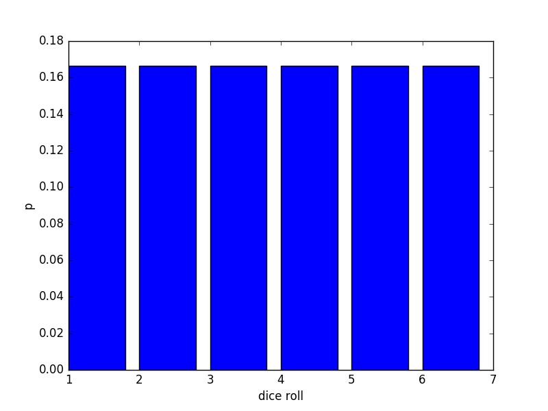
Let’s quickly run through some of the simplest cases. First, consider no constraints. Then \(p_i = e^{\lambda_0 - 1} = c\) To satisfy our the constraint that all probabilities sum to 1, then \(p_i= \frac{1}{n}\)
Now lets say that \(f_1(x) = x\), with \(<f_1(x)> = mu\) and \(f_2(x) = (x-mu)^2\) and \(<f_2(x)> = \sigma\). In other words, we know the mean and variance of \(p(x)\), but nothing else.
Then \(p(x) = e^{\lambda_0 - 1 + \lambda_1 x+ \lambda_2 (x-mu)^2}\)
A wild Gaussian has appeared! The condition that \(\int_{\mathbf{R}}p(x)dx\) be finite requires \(\lambda_1 = 0\) and \(\lambda_2 < 0\). After solving for the Lagrange multipliers we obtain: \(p(x) = \frac{1}{\sqrt{2\pi \sigma}} e^{\frac{(x-mu)^2}{2\sigma^2}}\)
The loaded dice
Let’s consider a “loaded dice”. The average number of dots returned from a fair dice is 21/6 = 7/2 = 3.5. Let’s suppose that we are told that instead we have a dice which yields an average of \(<p_i> = \mu\), where \(i\) is between 1 and 6. What is the MaxEnt prior for \((p_1, p_2, p_3, p_4, p_5, p_6)\)? First, we generalize to an \(n\) sided die, (at the end, we set \(n=6\).
From our above result, the unnormalized distribution is: \(p_i = e^{\lambda_0 - 1 + \lambda_1 i}\)
To get this in a nicer form, set \(e^{\lambda_0 - 1} = C\) and pull that constant out front: \(p_i = C e^{\lambda_1 i}\) Now set \(e^{\lambda_1} = r\): \(p_i = C r^i\) Now we have the normalization condition: \(\sum_{i=1}^n C r^i =1\) The left hand side is a geometric series: \(\sum_{i=1}^n r^i = \frac{r (r^n-1)}{r-1}\) Using this to find \(C\) we obtain: \(p_i = \frac{r-1}{r(r^n-1)} r^i\)
Now let’s solve for \(r\) in terms of \(\mu\) explicitly. We have the following condition: \(\sum_{i=1}^n\frac{r-1}{r(r^n-1)} i r^{i} = \mu\)
We need to know the following sum: \(\sum_{i=1}^n i r^i\)
This sum can be obtained by differentiating the sum of the geometric series. The result is \(\sum_{i=1}^n i r^i = \frac{nr^{n+2}-(n+1)r^{n+1}+r}{(r-1)^2}\)
The equation for \(r\) becomes: \(nr^{n+1}-(n+1)r^n+1= \mu(r^n - 1)(r -1)\)
Unfortunately, this equation doesn’t have any analytical solution, but it can be solved numerically, by finding the roots of: \((n-\mu)r^{n+1}+(\mu-n-1)r^n+\mu r-\mu+1=0\)
Let’s graph what \(p_i\) looks like. I wrote the following the Python code:
import numpy as np
import matplotlib.pyplot as plt
from scipy.optimize import fsolve

n = 6
mu = 2

func = \lambda r : (n-\mu)*r**(n+1) + (\mu-n-1)*r**n + \mu*r - \mu + 1

initial_guess = .3
r = fsolve(func, initial_guess)

index = np.zeros([n])
p = np.zeros([n])

for i in range(1,n+1):
index[i-1] = i
p[i-1] = ((1-r)/(1-r**n))*r**(i-1)

plt.bar(index, p)
plt.ylabel('p')
plt.xlabel('dice roll')
plt.show()
for \(\mu = 3.5\) we have:
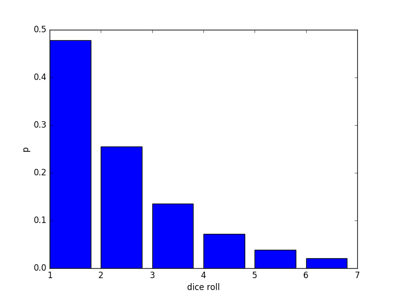
for \(\mu = 2\) we have:
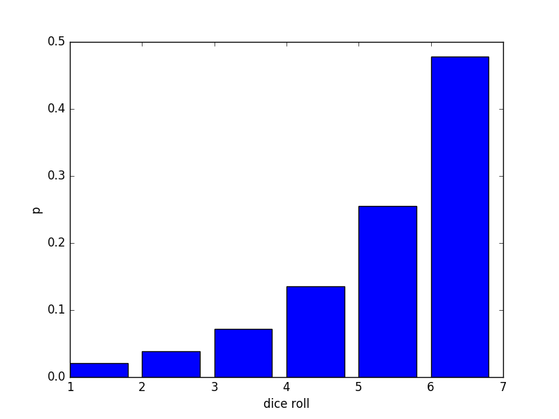
For \(\mu = 5\) we have:
For \(\mu = 5.9\) we have:
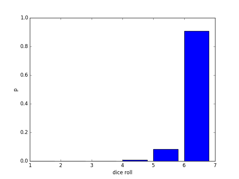
the algebraic computations were cumbersome, but it works!
Why some physicists love MaxEnt
MaxEnt is of interest to some physicists because it provides a framework for understanding the results of statistical mechanics as exercises in entropy maximization and inference. This connection was first described in a 1956 paper by E.T. Jaynes. Jaynes showed that statistical mechanics isn’t really “physics” at all. Semantically, one can draw a distinction between physical theory (ie. quantum mechanics), that can tell us the possible energy levels in a system, \(E_i\), and statistical mechanics, which is a framework for constructing a probability distribution \(P_i\) for the probability that the system is in state \(i\) given some (macroscopic) constraints. As the simplest example, we instance, we may know the average energy of the system.. In that case, we obtain the famous Boltzmann distribution for the canonical ensemble: \(p(i) = \frac{1}{Z}e^{-\beta E_i}\)
Where \(\beta = 1/T\). (for a full derivation, see here, pg. 27. Another slightly simpler exposition can be found here).
Different thermodynamic ensembles yield MaxEnt distributions, depending on the constraints imposed.
Does MaxEnt actually lead to any new that we didn’t already know from the textbook (ensemble) approach to statistical mechanics? No. For this reason, my phyicists are quick to dismiss it.
However, sometimes new frameworks allow us to push the boundaries of a theory in new directions (for example, the framework of Feynman path integrals allowed scattering amplitudes to be calculated which couldn’t be calculated before). In this case, physicists are interested in bridging the gap between equilibrium statistical mechanics and non-equilibrium stat mechanics. If you open a non-equilibrium statistical mechanics book, you will find non-equilibrium systems being tackled by two different approaches. In one approach, you will find methods that study small perturbations from the equilibrium case, such as the Boltzmann theory of transport for slightly out of equilibrium gases, and the popular theory of linear response. These approaches work good for understanding what happens when a few tracer molecules are introduced into a gas, or how a system responds when a small electric field that is turned on. These theories do not work very well for system which are far from equilibrium, such as living systems, or systems being driven by strong external fields. For such systems, one finds a collection of ad-hoc methods, which go under names such as master equations, memory functions, Langevin equation, and the generalized diffusion equation. There is a growing understanding that these ad-hoc methods can be understood as examples of MaxEnt being extended to the non-equilibrium case. When MaxEnt is extended to non-equilibrium case we have to consider all the trajectories a system can take through time, subject to some constraints. For instance, we may want to consider how a system may move from state A to state B. One considers the space of possible trajectories that meet these endpoint constraints, and construct a maximum-entropy distribution ( on this space of possible trajectories. This approach was first introduced by E.T. Jaynes in 1980 as the “principle of maximum entropy production”. He called the generalization “maximum calliber” (MaxCal). The calculations involved are very similar to Feynman path integrals, and can only be done explicitly for very simple systems (such as a driven harmonic oscillator). The cool thing with such calculations is that one can recover many of the ad-hoc equations of non-equilibrium stat mech. Therefore, there is growing optimism that MaxCal can help us learn fundamentally new ways of describing the behavior of out-of equilibrium systems.