Recently I experimented with decision trees for classification, to get a better idea of how they work. First I created some 2 dimensional training data with 2 categories, using sci-kit-learn:

import matplotlib.pyplot as plt
import numpy as np
from sklearn.datasets import make_moons, make_circles, make_classification

n_samples = 1000

X1, Y1 = make_classification(n_samples = n_samples, n_features=2, n_redundant=0,
 n_informative=2, n_clusters_per_class=1,
 class_sep=1, random_state=0)

X2, Y2 = make_moons(n_samples = n_samples, noise=0.3, random_state=0)

Next I wrote some code to test a decision tree with different numbers of splits for the two data sets:

def split(X):
 mid = len(X)//2
 return X[0:mid], X[mid:]

def plot_dt_vs_num_splits(X, Y, max_num_splits = 5, plot_step = .02):

 #split train and test data
 Xtrain, Xtest = split(X)
 Ytrain, Ytest = split(Y)

 #make meshgrid for plotting
 x_min, x_max = X[:, 0].min() - 1, X[:, 0].max() + 1
 y_min, y_max = X[:, 1].min() - 1, X[:, 1].max() + 1
 xx, yy = np.meshgrid(np.arange(x_min, x_max, plot_step),
 np.arange(y_min, y_max, plot_step))

plt.figure(2,figsize=(25,10))

splits = [1,2,5,10,100]
 num_splits = len(splits)

 for n in range(num_splits):
 dt = DecisionTreeClassifier(criterion = 'gini', max_depth=splits[n])
 dt.fit(Xtrain, Ytrain)

 #plot on mesh
 Z = dt.predict(np.c_[xx.ravel(), yy.ravel()])
 Z = Z.reshape(xx.shape)
 plt.subplot(1, num_splits, n+1)
 plt.contourf(xx, yy, Z, cmap=plt.cm.Paired)
 plt.scatter(X[:, 0], X[:, 1], marker='o', c=Y)
 plt.title("n_splits = " + str(splits[n]) +
 "\n train data accuracy = " + str(dt.score(Xtrain,Ytrain)) +
 "\n test data accuracy = " + str(dt.score(Xtest,Ytest)), fontsize=15)

plt.subplots_adjust(hspace=0)
 plt.axis("tight")
 plt.show()

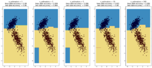
plot_dt_vs_num_splits(X1, Y1)
plot_dt_vs_num_splits(X2, Y2)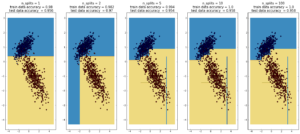

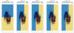
Here decision trees are exhibiting their classic weakness – so-called “high bias”, ie overfitting. Here, the tree was able to fit the data

first set of data (1000 points, 2 Gaussians) perfectly after 10 splits. In the case of the second data sets (1000 points, ‘moons’), the test data

accuracy decreases going from 10 to 100 splits, while the training data accuracy improves to 1, which is a sign of overfitting.

That is why people use boosted ensembles of trees. An ensemble is a weighted sum of models. In ensembles, many simple models can be combined to create a more complex one. The real utility of ensembles comes from how they are trained though, using boosting methods (wikipedia), which are a set of different techniques for training ensembles while preventing (or more technically delaying) overfitting.

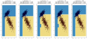
AdaBoost

(max depth of base estimators = 2) 

**

**

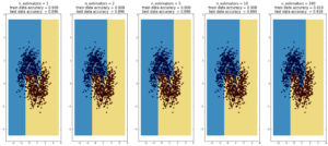
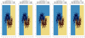
Random Forest

(max depth of base estimators = 2)

Random forest is currently one of the most widely used classification techniques in business. Trees have the nice feature that it is possible to explain in human-understandable terms how the model reached a particular decision/output.  Here random forest outperforms Adaboost, but the ‘random’ nature of it seems to be becoming apparent.. 

more commentary will follow.

Talks on boosted trees

Peter Prettenhofer – Gradient Boosted Regression Trees in scikit-learn

Trevor Hastie (a more detailed talk on Boosting / Ensembles)

MIT : boosting (a mishmash of general concepts)

Nando de Freitas : decision trees 

Nando de Freitas : Random forest